plumbing.data.blog

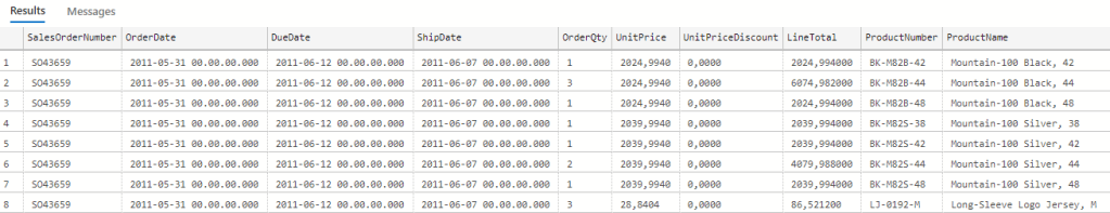
I’ve been toying with Azure Data Factory lately and especially with Data flows. It’s a graphical, low-code tool made for doing data transformations in cloud environment in a serverless manner. I got an idea of doing a little comparison between it and good old SQL from both performance and billing point of a view. My idea was to create a denormalized, a.k.a. wide table, by joining multiple tables together using both Data flows and SQL. I used AdventureWorks2019 sample database as a data source and combined 7 tables of sales related data and end result was like this:

Database I provisioned was the slowest and cheapest Azure SQL Database I could find: Basic tier which costs about whopping 4€ per month.

Result table contained 121 317 rows and the stored procedure, which populated it, was this:

SET ANSI_NULLS ON
GO
SET QUOTED_IDENTIFIER ON
GO
CREATE PROCEDURE [dbo].[uspCurated] 
AS
   SET NOCOUNT ON;
   
TRUNCATE TABLE dbo.curated_sp;

INSERT INTO dbo.curated_sp 
SELECT h.SalesOrderNumber, h.OrderDate, h.DueDate, h.ShipDate  
      ,d.OrderQty, d.UnitPrice, d.UnitPriceDiscount, d.LineTotal
      ,p.ProductNumber, p.name as ProductName
      ,pg.Name as ProductSubcategoryName
      ,pcg.Name as ProductCategoryName
      ,pm.Name as ProductModelName
      ,c.AccountNumber
FROM [Sales].[SalesOrderHeader] h
  INNER JOIN [Sales].[SalesOrderDetail] d on h.SalesOrderID=d.SalesOrderID
  INNER JOIN [Production].[Product] p on d.ProductID=p.ProductID
  INNER JOIN [Production].[ProductSubcategory] pg on p.ProductSubcategoryID=pg.ProductSubcategoryID
  INNER JOIN Production.ProductCategory pcg on pg.ProductCategoryID=pcg.ProductCategoryID
  INNER JOIN [Production].[ProductModel] pm on p.ProductModelID=pm.ProductModelID
  INNER JOIN [Sales].[Customer] c on h.CustomerID=c.CustomerID;
GO

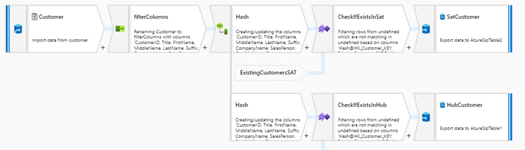
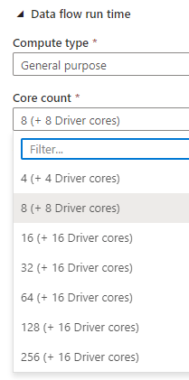
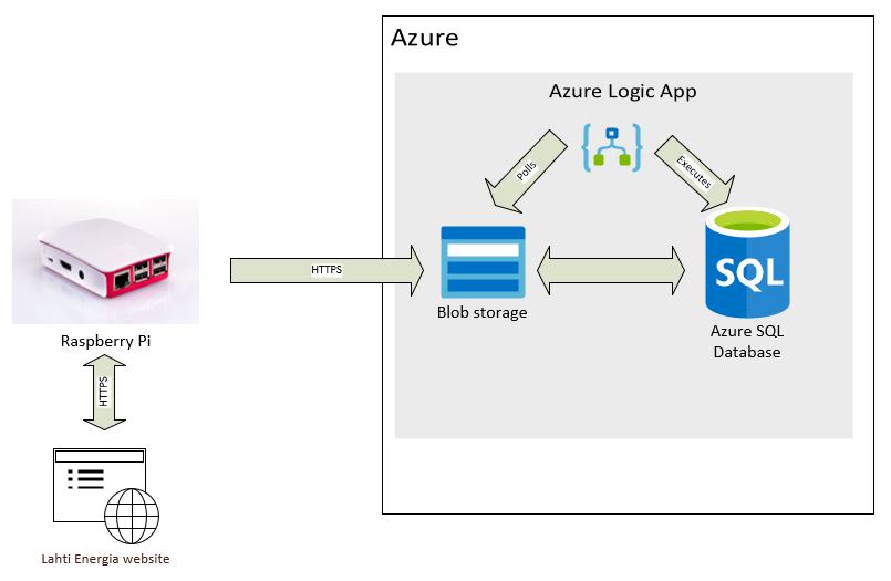
For Data flows I configured a runtime which type was General purpose and it had 8 cores. Pipeline I built is like the one below. Notice that not all sources are visible here but you get the idea:

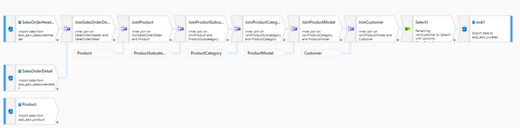
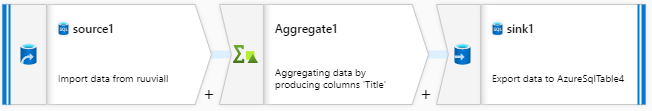
I used SalesOrderHeader as a starting point into which I joined other tables using Join transformation. Before saving end result back into database, there’s also a Select operator for filtering out unwanted columns after which the result set is pushed into table.

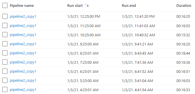
Both constructs (Data flow and Stored procedure) were placed into their own pipelines which both were scheduled to be run once in an hour for 1 day. So in total both ran 24 times. Here’s the statistics of running times in seconds:

Run Id	Duration (sec), Data flow	Duration (sec), Stored procedure
1	552	84
2	373	84
3	523	84
4	340	86
5	372	85
6	552	86
7	554	84
8	582	85
9	400	85
10	555	85
11	371	83
12	371	86
13	345	84
14	550	84
15	372	85
16	554	84
17	341	84
18	342	84
19	371	84
20	372	84
21	552	86
22	354	86
23	371	85
24	371	118
Average:	435	92

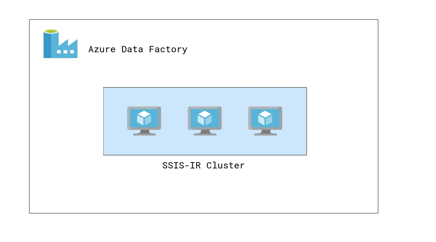
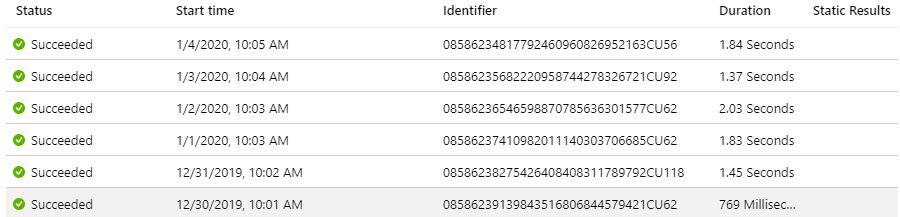
Stored procedure was both way more constant and a lot faster combined to Data flow. Let’s dive deeper into Data flow duration. What I found out was that warm up time of Spark cluster (which is technology behind Data flows) can be quite long. Here’s a sample of Run # 1 which took 9 minutes and 12 seconds to run in total. 5 minutes was spent just waiting for cluster to be ready:

Now that’s a long time! According to documentation, startup time varies between 4-5 minutes. In my test runs, which were done in Azure West Europe region, the average was approx. 3 minutes. Here’s the statistics but remember that your mileage may vary:

Run Id	Total duration (sec)	Cluster startup time (sec)	Actual runtime (total – startup)
1	552	298	254
2	373	102	271
3	523	282	241
4	340	96	244
5	372	130	242
6	552	290	262
7	554	303	251
8	582	326	256
9	400	140	260
10	555	284	271
11	371	103	268
12	371	126	245
13	345	103	242
14	550	289	261
15	372	130	242
16	554	291	263
17	341	92	249
18	342	103	239
19	371	103	268
20	372	109	263
21	552	307	245
22	354	103	251
23	371	98	273
24	371	97	274
Average:	435	179	256

Cluster startup times vary quite a lot from 1.5 minutes to 5 minutes. Actual runtime (the time from cluster being ready to end of execution) is much more constant. Using SQL we got all done in 1.5 minutes but just to get the Spark cluster up and running takes double!

Conclusions

If you already have your data in database then why not utilize its’ computing power to do data transformations? I mean it’s old technology and being old in this context is a good thing: Relational databases have been around more than 40 years which means those are well understood, well optimized and there’s a lot of scientific research behind those. Good old relational databases are still a valid solution for handling structured data.

Someone might say that test wasn’t fair and yes, I can relate to that. I mean data didn’t have to move out from SQL DB and then place back when using plain SQL. But then again should one move it to do some basic manipulations just that one could utilize some new and shiny low-code tool? I don’t think so: SQL is the lingua franca for data engineers and there’s a big pool of devs familiar with it.

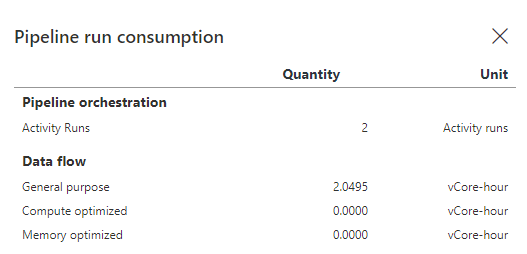
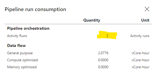
Even starting the Spark cluster took more time than getting things done with SQL. And guess what’s fun about this? You also pay for the cluster warmup time! But more of this and the whole cost of these two methods on part 2. Stay tuned!

Azure Data Factory is a cloud based tool for data movement and transformations. A little more than a year ago a new feature, Data flows, was published which made it possible to do data manipulations and transformations without coding: User can drag and drop components into canvas to build processes to move and transform data. There are different kind of components available for manipulating data like filter, pivot, aggregate and lookup. It’s a pretty nifty tool for a lazy data engineer. Here’s a picture of a Data flow which loads customer data into a Data Vault 2.0 modeled data warehouse:

Data flows are collected into pipelines which are a logical group of different activities. These together perform data manipulations. Under the hood Data flows are compiled and run on an Apache Spark cluster. According the documentation, pricing is based on three categories:

1. Type of compute
2. Number of cores in cluster
3. Running time

There are three different options for compute type to choose from:

1. General purpose: Default option and good for most workloads
2. Memory optimized for flows which have lots of lookups and joins (needs more memory)
3. Compute optimized for simple transformations

Cluster size can be configured while provisioning the runtime and minimum setup is 8 cores (16 for memory optimized). Here’s a list of available values for General purpose compute type:

At the time of writing (January 2021), the prices for different compute types in West Europe region are:

So if we have a Spark cluster which is of type General purpose, # of cores is 8 and we run it for one full hour, total cost will be 0,227€ * 8 = 1,816€. Pretty straightforward but let’s do test it anyway!

I created a dummy Data flow which connects to a Azure SQL database, aggregates data and saves result into database:

Then I set up a pipeline which ran this Data flow two times in a row. Don’t try to figure out the business logic of this ’cause there isn’t one: this is totally made up just to test the billing part:

A trigger ran this pipeline once in an hour for one day. Here’s a screenshot of monitoring view which shows couple of those runs. Interesting part from billing perspective is Duration column which tells us that the pipeline took approx. 16 minutes to finish:

Consumption details for each run can be viewed by pressing Consumption icon:

Details for the one above are here:

We can see that it took 2.0495 vCore hours to run. Where does this number come from? My runtime was a type of General purpose and had 8 cores in it. Total duration was 16 minutes which is about 0.2667 hours. And we had 8 cores so the total vCore-hours is 8 * 0.2667 which makes about 2.1. Quite close compared to 2.0495 shown above. There’s always some overhead in form of spinning up the cluster so actual run time of cluster is little less than total duration of pipeline. Price for this one run would be 2.0495 * 0.227€ which makes 0.47€.

In total pipeline ran 25 times. I went through those all and added vCore hours together and came up with a total of 52.0138. So the actual cost was 52.0138 * 0.227€ which makes 11.81€.

So far everything has been just a theory. How about reality? I mean what is the actual amount I’ll see in my bill? I was curious to see how this would look like so I jumped into Azure portal billing section. Here’s the result:

It shows 11.76€ so close enough compared to that 11.81€: Theory seems to work!

One thing to note in the billing data is the line cloud orchestration activity run which has a cost of 0.06€. Based on Data Factory billing documentation those refer to activity runs, trigger executions, and debug runs. Billing is based to number of these activities and price quite cheap: Less than 1€ for thousand activities:

So where does that 0.06€ in my bill come from? Let’s take a closer look at the picture of consumption details:

It has a row for Pipeline orchestration with an entry for Activity Runs and number two on it. Remember that in pipeline had two activities in it which both ran the same Data flow. That’s the reason for 2 activity runs. Pipeline was executed 25 times so number of activity runs is 25 * 2 = 50. Also all trigger executions must be added and there were 25 of those so the total number of activity runs in this case is 50 + 25 = 75. Now if we calculate the total amount, we will end up with figure 75/1000 * 0.844€ = 0.0633€. Once again close enough!

Conclusions

Data flow billing is quite straightforward and two main factors of cost are running time and size of the Spark cluster. There’s also some other things to be included but those are typically just a fraction compared to those two main factors.

Running classic SSIS packages in cloud has been possible for some time already. It is done utilizing Azure Data Factory (ADF) which contains a specific runtime engine called a SSIS Integration Runtime (SSIS-IR). Basically it’s just a cluster of Windows servers which are managed automatically by Azure. Those virtual machines have SSIS engine installed which is used to run SSIS packages.

• 

To reduce running costs, it’s a best practice to setup SSIS-IR to be on only when needed. In 2018 I was working in project in which we utilized SSIS-IR. I became curious about how long it takes to start up SSIS-IR so I setup a pipeline into ADF which just started and stopped SSIS-IR continuously. Based on these tests the average startup time was approx. 17,6 minutes.

Some time ago I bumped into a video in which a Microsoft representative announced that they had managed to speed up the starting process. Obviously it was time to rerun the tests. And indeed it is now much much faster than previously. Average time was now about 90 seconds. That means it’s now 10 times faster than previously. Here are the results visualized:

Both test runs contained about 100 full start-stop cycles. 2018 tests were run in Azure North Europe region, 2020 in West Europe. Node size D2_v3, number of nodes: 1. No custom configs.

But there’s a catch: Speedup only applies to those SSIS-IRs outside of a VNet! Inside the startup times are the same as previously, about 20 minutes on average. More details here.

Microsoft’s cloud ETL service, Azure Data Factory (ADF), has been in general availability for good time already. It’s a serverless platform for transforming and moving data between different kind of on-premise and cloud services. About year ago I was working as an architect in a project where we utilized ADF to move data into a blob storage. We had our blob attached to a VNET which means it was isolated from public network, effectively behind a firewall. VNET is a way to secure services so that those are not generally available to whole world. Problem then was the fact that connecting ADF to blob in a VNET was not possible without provisioning a virtual machine inside same VNET and installing a self-hosted integration runtime on it. We were building our solution in a serverless way so installing one didn’t sound like a great option.

Last fall things changed when Microsoft finally published a solution for connecting ADF into a storage account attached to a VNET. Now let’s see how it works!

For this demo I provisioned a Data Factory and two storage accounts:

Scenario is to copy a file from accestestsrc to accesstestdest. Source blob is public but destination is secured using VNET. Here’s how destination storage has been attached to a VNET so it is not accessible from everywhere:

Now let’s build a pipeline in Data Factory side to copy data from source to destination. While doing this, things go south when configuring destination sink:

Error 403 is thrown because ADF cannot connect to storage account because blob is connected to a VNET and ADF is not. To make connection happen we have to configure three things:

1. Add ADF’s managed identity into Storage accounts with proper access rights
2. Enable ‘Trusted Microsoft services’ setting on storage properties
3. Change authentication method from account key to managed identity

First one is done in storage account settings. Let’s select Access control (IAM) -> Add -> Add role assignment. For a Role we select ‘Storage Blob Data Contributor’ and then then name of our Data Factory (accessTestDataFactory) is written into ‘Select’ textbox. A query is done and our ADF will be listed below. Then we just select it and hit Save button.

Now our Data Factory is listed in assigned roles section:

Second part is done in Firewalls and virtual networks section. Select ‘Allow trusted Microsoft services to access this storage account’ and hit Save button. Azure Data Factory nowadays belongs to this set of Azure services which it wasn’t before announcement in fall 2019:

Lastly we have to change authentication method in ADF side: When we initially created connection to blob in ADF, it used account key as a method to authenticate. We must change it to use Managed identity to which we gave access rights to storage in step 1. Let’s edit linked service settings:

Now we are ready to finish and test copy pipeline again. It seems to complete without errors:

Let’s verify that the file has been actually copied to destination blob using Storage Explorer:

File somesuperimportantdatafile.txt is found in destination also so everything worked as planned.

I really like the simplicity this new feature enables. No more extra VM’s just to make connection happen and much more cleaner architectures. Also cheaper one because the absence of a VM. Go Serverless!

Last fall I got into playing with Ruuvitag sensors. Those are small, battery powered devices which measure temperature, humidity, pressure and acceleration. I placed one sensor to our sauna with and idea to make sauna call home: When certain temperature is reached, I’ll get a notification to my phone about sauna being ready to be utilized.

Ruuvitags are bluetooth beacons which broadcast measurements once in a second. Raspberry Pi has a bluetooth receiver built-in so it was a natural choice for listening the data stream. There is also a great Python library for Ruuvitags available which makes reading the measurements easy.

For notifications I’m utilizing Telegram messenger which I installed into my mobile. It’s an instant messaging app similar like WhatsApp or Signal. There’s a nice feature called bots which are basically third-party apps. The cool thing is that bots can be controlled using an API and that’s how I’m sending notifications to my phone. And there’s a Python library for Telegram also. What needs to be done in Telegram side is following:

1. Create a bot
2. Acquire token
3. Acquire chatid

There are multiple how-to documents available how to do this and here’s one.

I made a Python script which listens the Ruuvitag data stream, parses temperature out of it and if certain temperature is reached, it will send a notification. Script utilizes a file to store timestamp of when the latest notification was sent. This timestamp combined with resend timelimit parameter is for not flooding the phone with notifications:

from ruuvitag_sensor.ruuvi import RuuviTagSensor
from datetime import datetime
import telegram
import csv
import sys

# Two command line arguments:
# 1. Temperature limit
# 2. Resend timelimit in minutes

macs = [''] # MAC address of a Ruuvitag
timeout_in_sec = 10
temp_limit = float(sys.argv[1]) # Temperature limit (Celsius)  which indicates sauna being ready to enter
temperature = 0
resend_timelimit = float(sys.argv[2]) # Resend timelimit in minutes
now = datetime.utcnow()
dt_string = now.strftime("%Y-%m-%dT%H:%M:%S.%fZ")

# Let's fetch the latest measurement (timestamp and temperature):
reader = csv.reader(
   open("sauna.csv"), delimiter=";")
for row in reader:
   latest_notification = datetime.strptime(row[0], "%Y-%m-%d %H:%M:%S.%f")
   prev_temp = row[1]

# Fetching data from Ruuvitag:
data = RuuviTagSensor.get_data_for_sensors(macs, timeout_in_sec)

for j in data:
     temperature = data[j]['temperature']
     print('Measured temperature: '+str(temperature))
     print('Temperature limit: ' + str(temp_limit))
     datediff_in_minutes = (now - latest_notification).total_seconds() / 60 # time difference in minutes between now and when latest notification was sent
     print('diff in minutes: '+str(datediff_in_minutes))
     print('resend timelimit: ' + str(resend_timelimit))
     # IF temperature is above limit AND time difference between now and when latest notification was sent is more than resend timelimit THEN let's send a notification:
     if temperature >= temp_limit and datediff_in_minutes > resend_timelimit:
          # Let's create a Telegram bot
          bot = telegram.Bot(token='')
          chatid=
          chat_text = 'Sauna valmis! Lämpötila: ' + str(temperature)
          bot.send_message(chat_id=chatid, text=chat_text)
          f = open("sauna.csv", 'w')
          with f: # Let's write latest measurement into a file:
             writer = csv.writer(f, delimiter=";")
             writer.writerow([now, temperature])

MAC address of Ruuvitag must be placed into line 11. Lines 39-40 are for Telegram token and chatid.

Script is scheduled using cron. Below’s a screenshot of an actual notification.

Previous post was about utilizing cloud services to build processes. However I didn’t went all out on this: It was Raspberry Pi located at my home which was utilized to run Python code. And it is the weakest link from (at least) two point of view:

• Raspberry Pi’s SD memory card will eventually corrupt.
• Somebody has to maintain Raspberry Pi by patching the operating system and runtimes, monitor disk for not getting full etc. All the regular maintenance tasks administrators have to deal with. That somebody is me: Lazy data engineer.

I already had my first SD card corruption happened last fall: It took only two years from purchase to occur. Second bullet point is much more general problem and it covers all on-premise systems and IaaS option in the cloud as well: Maintenance overhead. One option to avoid SD corruption could be utilizing a VM running on Azure. But then again there’s a problem with bullet point two: Somebody has to maintain that VM. I wish there was a service into which I could just submit the code and not worry about this kind of things…

And there is: Azure has services for building business processes in cloud without having to worry about the server(s) running it. This concept is called serverless. It’s a little bit misleading term since actually there are servers under the hood but the main point is that developers don’t have to worry about those. Traditionally difficult problems, like scaling, is taken care of by the platform so developers can focus on the main thing: Building business processes. Serverless also means apps are billed only when those are actually run so no cost is generated when there isn’t usage. This is called a consumption based plan. So it’s like bring-your-own-code-and-don’t-worry-about-the-platform®.

Serverless offering in Azure builds on top of Logic Apps and Azure Functions. First one is a service for building workflows using a visual designer to automate business processes without coding. It has lots of built-in connectors available for both cloud and on-premise systems and services. It’s based on triggers which means a workflow is kick-started when something happens, e.g. a timer is hit, an certain event (like a file landing into a blob container) happens or a HTTP request is received.

Azure Functions is a service for running code in cloud environment. Language choices at the time of writing are C#, F#, Python, JavaScript, Java, PowerShell and TypeScript. Check the official documentation.

Usually Logic Apps and Functions goes hand in hand so that Logic App works like an orchestrator and calls different functions to control the flow of business processes.

The architecture I was aiming at was like this: Getting rid of Raspberry Pi and setting up a Azure Function to run existing Python code:

Python is one of supported languages so that was a natural choice since original code was written on it. It turned out so that all changes I had to do was how to schedule it and how to interact with storage account.

Scheduling can be done using triggers. One type of those is a timer and it’s the one used here. There are also other types of triggers available like an event based (e.g. file lands into blob).

Connecting the function to storage account is achieved using bindings which are endpoints to different Azure services like blob storage, Event Hubs, Cosmos DB etc. In this case we are uploading a csv file to blob so it’s an output binding. To get data into a function, one can use input bindings. Check the documentation for details.

Triggers and bindings are configured in a file named function.json which in this case was like this:

{
  "scriptFile": "__init__.py",
  "bindings": [
    {
      "name": "mytimer",
      "type": "timerTrigger",
      "direction": "in",
      "schedule": "0 0 8 * * *"
    },
    {
      "type": "blob",
      "direction": "out",
      "name": "outputBlob",
      "path": "sahko/inputdata.csv",
      "connection": "AzureWebJobsStorage"
    }
  ]
}

Mytimer is a schedule for running the function and described as a NCRONTAB expression. It’s like a classic CRON except having an extra sixth field at the beginning which describes seconds (original CRON has time granularity at minute level). Schedule is 0 0 8 * * * which means the function is run in the morning at 08:00 every day. OutputBlob is a binding to storage account container/filename (sahko/inputdata.csv).

Here’s the actual Python code:

import os
import requests
from lxml import html
from datetime import datetime, timezone
from azure.storage.blob import BlobServiceClient
import azure.functions as func

def main(mytimer: func.TimerRequest, outputBlob: func.Out[str]) -> None:
 
    LOGIN = os.environ["LOGIN"]
    PASSWORD = os.environ["PASSWORD"]
    LOGIN_URL = os.environ["LOGIN_URL"]
    URL = os.environ["URL"]

    session_requests = requests.session()

    # Get login csrf token
    result = session_requests.get(LOGIN_URL)
    tree = html.fromstring(result.text)
    authenticity_token = list(set(tree.xpath("//input[@name='__RequestVerificationToken']/@value")))[0]

    # Create payload
    payload = {
        "username": LOGIN,
        "password": PASSWORD,
        "__RequestVerificationToken": authenticity_token
    }

    # Perform login
    result = session_requests.post(LOGIN_URL, data = payload, headers = dict(referer = LOGIN_URL))


    # Scrape url
    result = session_requests.get(URL, headers = dict(referer = URL))

    formatted_output = result.text.replace('\\r\\n', '\n')

    for line in formatted_output.splitlines():
        if line.lstrip()[0:11] == 'var model =':

            jsonni = line.lstrip()[12:-1]
            start = jsonni.find('[[')
            end = jsonni.find(']]')
            jsonni = jsonni[start+1:end+1]
            jsonni = jsonni.replace('],[','\n')
            jsonni = jsonni.replace(']','')
            jsonni = jsonni.replace('[','')

            output = 'timestamp;consumption\n' # header for csv-file
            for line in jsonni.splitlines():
                start = line.find(',')
                epoc = line[0:start]
                measure = line[start+1:]
                timestamp = int(epoc)/1000
                timedate = datetime.fromtimestamp(timestamp, timezone.utc)
                timestamp_str = str(timedate)[:-6]
                output += timestamp_str + ';' + measure + '\n'

            outputBlob.set(output)

On line 8 one can see how timer trigger and output binding are utilized. Line 59 shows how to write csv file into blob. I also took the hard coded connection strings, urls, user id and password away from the code file into application settings. Those values are fetched on lines 10-13.

All other sections are identical compared to original code so in that sense it can be said it was pretty straightforward to migrate existing application from on-premise to serverless.

Development was done using Visual Studio Code. One thing to note is that setting up Azure Function & Python environments in VS Code was a painful experience and could be a blog post on its own.

Solution has been running as serverless now for two weeks without problems. Here’s a screen shot of Azure Portal of actual execution logs. It takes about 5 seconds for code to run:

Originally I planned it so that Logic App would do orchestration of all components. I mean Logic App would also call Function based on a timer which is set up in Logic App side. However this didn’t work as I initially planned since at the moment Logic App only supports calling Functions which use .NET or JavaScript as a runtime stack. Most likely this will change in future and also Python (and other languages not supported at the moment) functions can be utilized from Logic Apps. And when this happens, there will be a blog post about it!

I wanted to monitor our electricity usage on more granural timeframe than the monthly bills we are getting. My local provider Lahti Energia has usage statistics available on their website that are on a hourly granularity. It even has some data visualizations built-in but those are kind of basic so I figured I could build something by myself.

It is possible to download data in a csv format but that requires logging into service and manually doing some selections. As a lazy data engineer I want to automate things. Unfortunately there’s no any kind of an API, like REST, available so I had to come up something else: Web scraping. It is a method where web browsing is done programmatically to get the data needed. It’s far from ideal because even a tiny change in web page can break the procedure. But since there wasn’t API available, scraping was the way forward.

I had Raspberry Pi up and running so I figured a Python script could do the heavy liftin’n’shiftin. Python also has lots of good libraries for doing screen scraping, connecting Azure etc.

I wanted to utilize cloud services as much as possible because I like the concept of someone else taking care of the platform. So I decided to place the data into a relational cloud database: Azure SQL DB. I already had one running so it was only a matter of creating a couple of database objects. I also like to minimize the amount of code and that’s why utilizing Azure Logic App to orchestrate whole thing seemed to be a right choice.

The architecture I came up is as follows:

1. Python script running on my Raspberry Pi scrapes the electricity usage data from my local provider’s web site.
2. Script parses data into tabular format (good old csv) and places the file into a specific Azure blob storage container. Script is scheduled using cron.
3. Azure Logic app is setup so that it polls blob storage container for new files. When a new file is found, it kicks up a stored procedure found from Azure SQL DB which imports the file into a staging table and from there all new rows are inserted into actual table.

For doing screen scraping against website that requires login, I followed this handy tutorial: https://kazuar.github.io/scraping-tutorial/. Also a big shout out to stackoverflow.com for providing lots of good code examples e.g. how to connect Azure storage, convert UNIX epoch time to timestamp etc.

Microsoft has lots of Python modules for managing Azure services and I’m utilizing those to connect Storage account. I already had a storage account so it was just a matter of creating a new container on it and getting a connection string. A parameter connection_string is a pointer to a storage account and it can be found from Azure Portal -> Storage account -> Access keys -> Connection string.

Actual usage data can be found from web page source from a line which begins with a string ‘var model =’. Value is a JSON object but not actually a valid one. This is parsed to tabular format with two column: Timestamp and consumption.

Here’s the code I ended up using:

import requests
import csv
from lxml import html
from datetime import datetime, timezone
from azure.storage.blob import BlobServiceClient

connection_string = "DefaultEndpointsProtocol=https;AccountName=...

# Create the BlobServiceClient object which will be used to create a container client
blob_service_client = BlobServiceClient.from_connection_string(connection_string)

# Create a blob client using the local file name as the name for the blob
blob_client = blob_service_client.get_blob_client(container='sahko', blob='inputdata.csv')

USERNAME = ""
PASSWORD = ""

LOGIN_URL = "https://online.lahtienergia.fi/eServices/Online/Login"
URL = "https://online.lahtienergia.fi/Reporting/CustomerConsumption?loadLastMonthData=true"

def main():
    session_requests = requests.session()

    # Get login csrf token
    result = session_requests.get(LOGIN_URL)
    tree = html.fromstring(result.text)
    authenticity_token = list(set(tree.xpath("//input[@name='__RequestVerificationToken']/@value")))[0]

    # Create payload
    payload = {
        "username": USERNAME,
        "password": PASSWORD,
        "__RequestVerificationToken": authenticity_token
    }

    # Perform login
    result = session_requests.post(LOGIN_URL, data = payload, headers = dict(referer = LOGIN_URL))
    #print(result.content)

    # Scrape url
    result = session_requests.get(URL, headers = dict(referer = URL))

    formatted_output = result.text.replace('\\r\\n', '\n')

    for line in formatted_output.splitlines():
        if line.lstrip()[0:11] == 'var model =':
            jsonni = line.lstrip()[12:-1]
            start = jsonni.find('[[')
            end = jsonni.find(']]')
            jsonni = jsonni[start+1:end+1]
            jsonni = jsonni.replace('],[','\n')
            jsonni = jsonni.replace(']','')
            jsonni = jsonni.replace('[','')

            with open('usagedata.csv', 'w', newline='') as file:
                writer = csv.writer(file, delimiter=';') # Let's also write data into file
                output = 'timestamp;consumption\n' # header for csv-file
                for line in jsonni.splitlines():
                    start = line.find(',')
                    epoc = line[0:start]
                    measure = line[start+1:]
                    timestamp = int(epoc)/1000
                    timedate = datetime.fromtimestamp(timestamp, timezone.utc)
                    timestamp_str = str(timedate)[:-6]
                    writer.writerow([timestamp_str, measure])
                    output += timestamp_str + ';' + measure + '\n'
            blob_client.upload_blob(output,overwrite=True)

if __name__ == '__main__':
    main()

The csv file is given a name inputdata.csv and is placed into a container named sahko. It has two columns separated by a semicolon: timestamp and comsumption which tells the electricity consumption during that hour:

timestamp;consumption
2019-12-04 00:00:00;0.3
2019-12-04 01:00:00;0.06
2019-12-04 02:00:00;0.29
2019-12-04 03:00:00;0.06
2019-12-04 04:00:00;0.24
2019-12-04 05:00:00;0.12
2019-12-04 06:00:00;0.23
2019-12-04 07:00:00;0.23
2019-12-04 08:00:00;0.21
2019-12-04 09:00:00;0.3
2019-12-04 10:00:00;0.07
2019-12-04 11:00:00;0.31
2019-12-04 12:00:00;0.06

Now we have raw data stored in blob! To get the csv file from blob to SQL, these two services must be connected. First a shared access signature (SAS) to blob needs to be created. After SAS being created, following commands are being run in Azure SQL DB:

CREATE MASTER KEY ENCRYPTION BY PASSWORD = '...';

CREATE DATABASE SCOPED CREDENTIAL MyCredentials WITH IDENTITY = 'SHARED ACCESS SIGNATURE',SECRET = 'st=...';

CREATE EXTERNAL DATA SOURCE MyAzureStorage WITH (
TYPE = BLOB_STORAGE,
LOCATION = 'https://<storage_account_name>.blob.core.windows.net',
CREDENTIAL = MyCredentials
);

First command creates a master encryption key. Choose a strong password. After this a stored credentials can be made which utilizes the shared access signature created earlier. Lastly an actual external data source can be created utilizing these stored credentials to connect storage. To verify the connection, following SQL query can be run:

Now the Azure SQL DB is successfully connected into storage! Now let’s create a stored procedure dbo.sp_insert_data for loading csv file into a database table:

CREATE PROCEDURE [dbo].[sp_insert_data]

AS
BEGIN

	TRUNCATE TABLE [dbo].[stg_sahko];

	BULK INSERT [dbo].[stg_sahko]
	FROM 'sahko/inputdata.csv'
	WITH (DATA_SOURCE = 'MyAzureStorage',
		  FIELDTERMINATOR = ';',
		  ROWTERMINATOR = '0x0a', --LF
		  FIRSTROW = 2);

	INSERT usage(pvm, usage)
	SELECT CAST(s.[pvm] AS DATETIME) AS pvm
          ,CAST(s.[usage] AS NUMERIC(10,2)) AS usage
	FROM stg_sahko s LEFT JOIN usage u ON s.pvm=u.pvm 
	WHERE u.pvm IS NULL;
    
END
GO

The logic goes so that first a temporary staging table (dbo.stg_sahko) is emptied by running a truncate command. Then raw data from csv file is loaded into this table. We have to tell a little bit of metadata (field terminator character, row terminator and first row) so that the database engine knows how to load file correctly. From staging table only new rows are loaded into actual destination table (dbo.usage) and also the fields are casted into real datatypes (datetime & numeric).

Now we have methods for both generating a csv file and loading that into database. Now we just have to combine there two so that when csv file is placed into blob, it will be loaded into database. For this I’m utilizing Azure Logic app which is a service for automating and orchestrating data flows, processes etc.

Azure Logic app acts like an orhestrator: It polls the specific container (sahko) in blob storage and if there’s new file added (or modified), it fires stored procedure located in SQL to load data into table. Here’s the workflow:

• 

Python script runs once a day at 10 am and pushes the csv file into blob. Even though the website data has a granularity of one hour, it is only updated once a day so there’s no point running script more than once a day.

Here’s a screen shot of Logic App logs which shows that the stored procedure has been run couple minutes after csv file has landed into blob container:

Here’s a screenshot of actual target table in SQL:

And that’s it folks! I’ve shown how to automate data gathering utilizing modern cloud services. I didn’t touch the area of data analysis at all but let’s see if we are able to do that on following posts.